
Just like Microsoft's Excel, Google Sheet has equally powerful functions hidden up its sleeve. It can help you do routinary, mundane tasks fast and perform time-saving complex operations.
With Google Sheet, being an open-source software and with its collaboration support, it's likely that you'll end up using the app more often than not. It's one indispensable tool every web master and virtual assistant can't live without.
While you may not use below's list of useful Google Sheet functions everyday, it pays to be familiar and well-verse with these shortcuts. We hand-picked this shortlist of five essential Google Sheets hacks to help you save time in dealing with spreadsheets.
1. Use SPLIT function and obtain the first word from a phrase
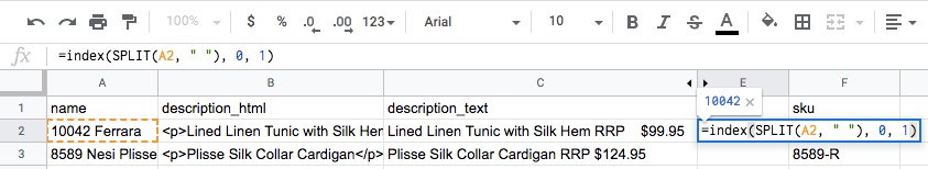
Suppose you want to extract the first word from a string in a Google Sheet column. You can use SPLIT() function to split a string and obtain first word , as follows:
=index(SPLIT(A2, " "), 0, 1)
With the above function, a string “10042 Ferrara” yields “10042”.
To obtain the n word, just replace 1 with n accordingly.
2. Use REGEXEXTRACT to retrieve number from a string
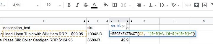
Suppose you have this data in a column and you wish to obtain the price
<p>Lined Linen Tunic with Silk Hem</p><p> </p><p><strong>RRP $99.95</strong></p>
You can do so with REGEXEXTRACT function to extract the price, as follows:
=REGEXEXTRACT(C2, "[0-9]*\.[0-9]+[0-9]+")
3. Using CONTACT to combine multiple values
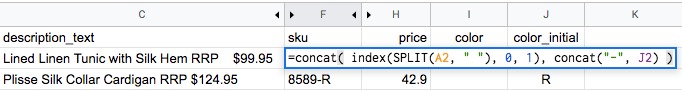
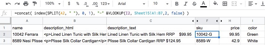
Suppose in Column A you want to get the first word and combine it with the value in Column J, you can achieve it using CONCAT function.
=concat( index(SPLIT(A2, " "), 0, 1), concat("-", J2) )
Or use ampersand to combine multiple values:
="RRP "&value(REGEXEXTRACT(E12, "[0-9]*\.[0-9]+[0-9]+"))
4. Use SUBSTITUTE() & RegexReplace() to search and replace
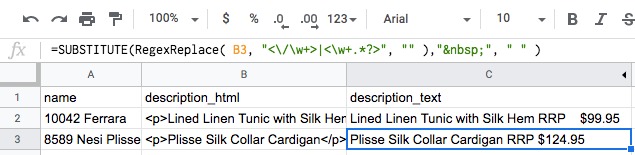
Say you have a column of data that contains HTML ASCII codes and you want to get rid of them. Here's how you do it:
=SUBSTITUTE(B2," ", "")
Or you can go creative, do a nested SUBSTITUTE
=SUBSTITUTE(SUBSTITUTE(B2, "</p>", ""),"<p>", "")
Or you can go use RegExReplace to get rid all HTML tags
=RegexReplace( B2, "<\/\w+>|<\w+.*?>", "" )
Or a combination of Substitute and RegexReplace
=SUBSTITUTE(RegexReplace( B3, "<\/\w+>|<\w+.*?>", "" )," ", " " )
3 Things You Didn't Know Google Spreadsheet Can Do For You (Part 1)
5. Use VLOOKUP to search by keyword and return a specified cell from another sheet
Google Sheet's vertical lookup is a powerful function you need to master. It lets you search down the first column of a range for a key and returns the value of a specified cell in the row found.
If that doesn't make sense, imagine you have Sheet14 containing sku and color columns
 Sheet14
And wanted to append the color initial found inside a separate table from Sheet15
 Sheet15
You can do a quick search using VLOOKUP and return the color initial (from Sheet15) by providing color from Sheet14.
The full formula:
=VLOOKUP(I2, Sheet15!A1:B7,2, false)
Where I2 is the keyword, Sheet15!A1:B7 is the range, and 2 is column position from Sheet15 we want to retrieve.
Excel Gets OCR Support, Lets You Snap Tables and Convert Into Editable Spreadsheet
So next time you are asked to update a Google Sheet and do dead boring, repetitive tasks, try to look around inside Google Sheet list of functions and see if you can automate stuff and save huge amount of time in the process.


